
VLOOKUP was one of the first functions I learned. As I began using it, I felt like a superhero!
What it does: VLOOKUP searches for specific data in a data table. VLOOKUP searches vertically for specific data in the left-most column in a data table (hence the “V”) and returns the data found at a specific offset to the right, in the same row where the Lookup_value is found. I know it sounds a bit confusing, but hang with me, it’ll become clearer and you’ll be saving lives in no time!
Syntax: =VLOOKUP(Lookup_value,Table_array,Col_index_num,Range_lookup)
|
Element |
Description/Treatment |
| Lookup_value: |
This is required. This is the item to be found in the left-hand column of the “Table_array”. The Lookup_value determines the row from whence the data to the right will be pulled. If the Lookup_value is not found in the far-left-most column, the function will return a #N/A error. The Lookup_value can be a number, reference, named range or text string.
|
| Table_array: |
This is required. This is a range of data wherein the left-most column is used for the “Lookup_value”. The left-most column is always searched first, vertically. Data is pulled from the columns to the right of the Lookup_value in the same row where the Lookup_value is found. ***Save Your Life Tip *** If/When possible, use named ranges for your Table_array. Also, if you “fill” the function over many cells and you do not use named ranges, you must anchor (using “$” or toggle through the F4 key) your Table_array. Otherwise, your Table_array will be dynamic and will change for each row/column to which you “fill”. |
| Col_index_num: |
This is a number that tells the function from which column to the right to pull data (Offset column). The left-most column is always “1” (sans quotes). If you use a number that is greater than number of columns in the Table_array, you’ll get a #REF! error. You cannot use negative numbers. |
| Range_lookup: |
This is an optional element of the function. This is a precision switch and is either True or False. If you want an approximate (close enough) result, select True. The approximate result means that the result is the largest item that doesn’t exceed the Look_up value. If you want an exact result, select False. You can substitute 1 for True and 0 for False and the function will work just fine. As the Range_lookup is optional, it can be omitted. If omitted, the default will be used. The default is True (e.g. approximate match), which frankly, is dangerous unless you know that close enough is good enough… I almost never use the “True” option, although to not use the “True” feels counterintuitive to me. |
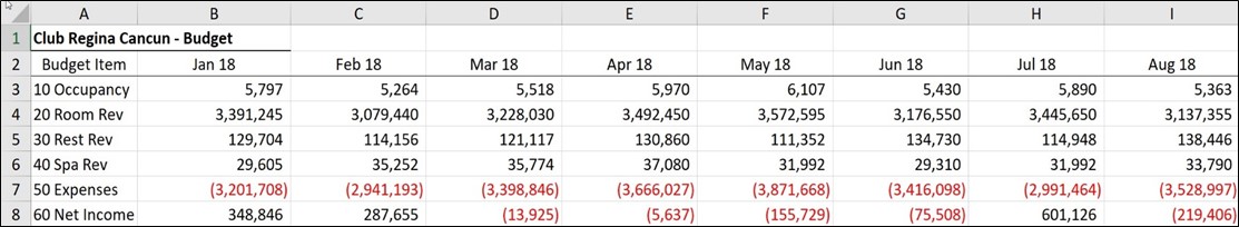
- Say we wanted to pull the July 2018 Room Revenue, the formula would look like:
|
Formula |
Result |
| =VLOOKUP(“20 Room Rev”,A3:I8,8,FALSE) |
3,445,650 |
|
Element |
Description/Treatment |
| Lookup_value: |
“20 Room Rev” This is a text string that Excel will look for in the far-left column of the Table_array. |
| Table_array: |
A3:I8 This is the range for which Excel will search vertically in the far-left column (e.g. A3:A8), then returns the data from the columns to the right (B3:I8). |
| Col_index_num: |
8 This is the column offset for the period we want to see (e.g. July) Although July is the 7th month, because the first column in the Table_array is the Budget Item, the Col_index_num needs to account for the additional column (7 (July) plus 1 (Budget Item Column) = 8). |
| Range_lookup: |
False As this is an optional element of the function, I’ve selected an exact match. |
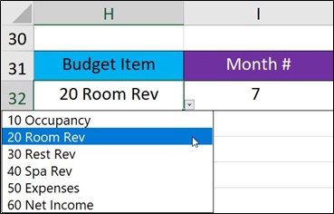
- Or, say we used data validation, a named range and a month selector, the formula would look like:
|
Formula: |
Result: |
|
=VLOOKUP(H32,ClubReginaCancun2018Budget,I32+1,0) |
3,445,650 |
The data validation and the month selector ranges are:
|
Element |
Description/Treatment |
| Lookup_value: |
H32 This is a reference to cell H32 as a data validation selection. Excel will look for the contents of H32 in the far-left column of the Table_array. |
| Table_array: |
ClubReginaCancun2018Budget This is a named range that refers to cells A3:I8. The Table_array includes the vertical lookup range in the far-left column (e.g. A3:A8), then returns the data from the columns to the right (B3:I8). |
| Col_index_num: |
I32+1 This is reference to add 1 to the contents of cell I32. I32 is the number reference for July (7). Although July is the 7th month, because the first column in the Table_array is the Budget Item, the Col_index_num needs to account for the additional column (7 (July) plus 1 (Budget Item) = 8). |
| Range_lookup: |
False As this is an optional element of the function, I’ve selected an exact match. |
Leave a Reply